training an image consistency model from scratch

2025-11-22

I had some free time a few weeks ago and trained an image consistency model from scratch to see how cool it would be. As expected, it’s a fun experience. So, I’ll be plotting down whatever I learnt during the training phase.

Generally, diffusion models are used to generate high-fidelity visuals with expensive computation and denoising steps. To overcome this, OpenAI introduced “Consistency Models” that can generate high-quality samples in a single step and even better samples with multi-step sampling.

Github - https://github.com/Abinesh-Mathivanan/beens-image-gen

Part 1 - Diffusion vs Consistency models.

A diffusion model is trained to reverse a process that gradually adds noise to an image. This forward process is defined by a stochastic differential equation (SDE) that takes a clean image $x_0$ and produces a noisy version $x_t$ at time $t$. The model’s job is to learn the score function: $$\nabla_x \log p_t(x)$$ This is a vector field that points in the direction of increasing data density. During inference, a reverse-time SDE solver uses this score function to guide a random noise sample $x_t$ back towards the distribution of clean images, step by step: $$x_t \rightarrow x_{t-\Delta t} \rightarrow \dots \rightarrow x_0$$

In short, A diffusion model learns to take one small step at a time. It’s an expert at predicting the noise at a specific time $t$ to get to $t-\Delta t$.

Meanwhile, the Consistency model works by the principle:

Instead of learning a step-by-step transition, it is trained to map any noisy point $x_t$ on a trajectory directly back to the trajectory’s origin, the clean image $x_0. This is called the consistency property. Mathematically, a function $f$ is a consistency model if it satisfies:

Consistency Property: For any time $t, t’ \in [\epsilon, T]$ and any pair of points $x_t$, $x_{t’}$ on the same trajectory, $$f(x_t, t) = f(x_{t’}, t’) = x_0$$ Here, $\epsilon$ is a minimum noise level (close to 0) and $T$ is the maximum.

If the model is truly consistent, it doesn’t matter how much noise you have ($t$); it should always be able to identify the original image in a single shot. This is why it can perform one-step generation: just give it pure noise $x_T$ at the maximum timestep $T$, and $f(x_T, T)$ should directly yield the final image.

The training objective is designed to enforce this property. The loss function is approximately: $$L(\theta, \theta^{-}) = \mathbb{E}[d(f(x_{t_{n+1}}, t_{n+1}; \theta), f(x_{t_n}, t_n; \theta^{-}))]$$

Where:

$\theta$ are the weights of the online (“student”) model.
$\theta^{-}$ are the weights of the EMA (“target”) model.
$x_{t_n}$ and $x_{t_{n+1}}$ are two adjacent points on a noise trajectory.
$d$ is a distance metric (like L1 or L2 loss).

Part 2 - Architecture

At the core, we’ll go with U-Net (a symmetric encoder-decoder structure with skip connections which preserves high-resolution spatial information).

I explain the whole process in short:

Timestep Embedding: The network is told how much noise it’s dealing with before the image input. The simple number that represents the noise level (the time step $t$) is converted into a special embedding.
The Encoder: The noisy image starts at its full size ($64 \times 64$). This path squeezes the image down to smaller and smaller sizes (like $32 \times 32$, $16 \times 16$, $8 \times 8$) and learns the big picture. Also it saves a copy of the full-features in the form of skip-connections
Middle Block: The image is now at its smallest, most abstract form ($8 \times 8$) and high-level features are captured.
The Decoder: The network starts building the image back up to its original size. At each level of upsampling (e.g., $8 \times 8 \rightarrow 16 \times 16$), it pulls in the corresponding skip connection. This is like looking at the rough sketch and then immediately checking the saved details to make sure the final output is accurate. This process restores the fine-grained details.
Output: Once the image is back to its original size, the last layer simply adjusts the features to output the final result. The result is the network’s best guess at the amount of noise that needs to be subtracted to get a cleaner image.

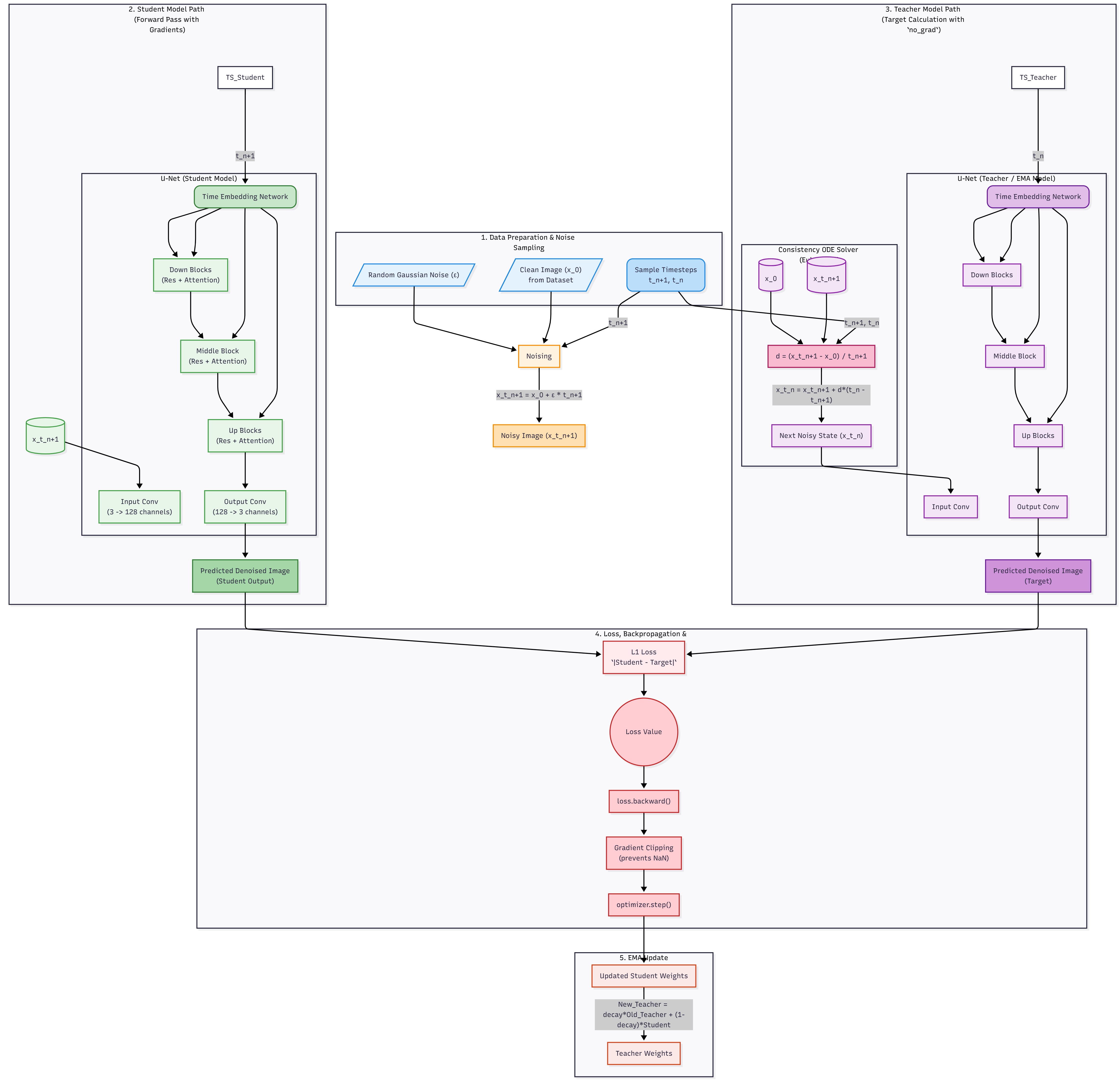
Consistency Architecture diagram

2.1 - Timestep embedding:

The model needs to know the noise level (or “time,” $t$) of the image it’s currently processing. Using a simple scalar number won’t be a very reliable input. So, We solve this by converting the scalar t into a high-dimensional vector using sinusoidal embeddings (adds positional encodings to embeddings at the start of encoder / decoder).

A set of fixed frequencies (freqs) is created.
Each input timestep ($t$) is multiplied by every frequency.
The $sin$ and $cos$ of these values are calculated and concatenated.

1
def timestep_embedding(timesteps, dim, max_period=10000):
2
    half = dim // 2
3

4
    freqs = torch.exp(-math.log(max_period) * torch.arange(start=0, end=half, dtype=torch.float32) / half).to(device=timesteps.device)
5

6
    args = timesteps[:, None].float() * freqs[None]
7
    embedding = torch.cat([torch.cos(args), torch.sin(args)], dim=-1)
8

9
    if dim % 2:
10
        embedding = torch.cat([embedding, torch.zeros_like(embedding[:, :1])], dim=-1)
11

12
    return embedding

2.2 - The Conditional ResBlock

This residual block that processes the image features, but with a crucial addition: it’s conditioned on time.

The input image feature map $x$ passes through a normalization, activation (SiLU), and convolutional layer.
Simultaneously, the timestep embedding emb is passed through its own small neural network (emb_layers) to project it into a format that can interact with the image features.
This projected embedding is added directly to the image features. This is the conditioning step we’re talking about. It allows the network to modulate its behavior based on the noise level $t$.
The combined feature map passes through the second half of the block.
At last, we implement a residual connection that adds the original input $x$ to the output, supporting gradient flow and stabilizing training.

1
class TimestepBlock(nn.Module):
2
    pass
3

4
class ResBlock(TimestepBlock):
5
    def __init__(self, channels, emb_channels, dropout, out_channels=None, use_scale_shift_norm=False):
6
        super().__init__()
7
        self.out_channels = out_channels or channels
8
        self.in_layers = nn.Sequential(
9
            nn.GroupNorm(32, channels),
10
            nn.SiLU(),
11
            nn.Conv2d(channels, self.out_channels, 3, padding=1)
12
        )
13

14
        # process the timestep embedding
15
        self.emb_layers = nn.Sequential(
16
            nn.SiLU(),
17
            nn.Linear(emb_channels, self.out_channels)
18
        )
19

20
        self.out_layers = nn.Sequential(
21
            nn.GroupNorm(32, self.out_channels),
22
            nn.SiLU(),
23
            nn.Dropout(p=dropout),
24
            nn.Conv2d(self.out_channels, self.out_channels, 3, padding=1)
25
        )
26

27
        # skip connection to match input/output channels if they differ
28
        self.skip_connection = nn.Conv2d(channels, self.out_channels, 1) if channels != self.out_channels else nn.Identity()
29

30

31
    def forward(self, x, emb):
32
        # process the image features
33
        h = self.in_layers(x)
34

35
        # process the timestep embedding
36
        emb_out = self.emb_layers(emb).type(h.dtype)
37

38
        # add the embedding to the image features
39
        # we expand the embedding to match the spatial dimensions of h
40
        h = h + emb_out[..., None, None]
41

42
        # process through the rest of the block
43
        h = self.out_layers(h)
44

45
        # add the residual connection
46
        return self.skip_connection(x) + h

2.3 - Attention Block

To understand long range dependencies, we implement a Self-Attention Block

The input feature map $x$ is flattened from (B, C, H, W) to (B, C, H*W), treating each pixel location as a “token.”
Query, Key, and Value vectors are created from this sequence using a Conv1d layer (which acts like a Linear layer on each token).
The standard attention mechanism computes a weighted average of the Value vectors, where the weights are determined by the similarity between Query and Key vectors.
This allows a pixel in one part of the image to directly gather information from any other pixel, regardless of distance. The output is added back to the input (a residual connection) and reshaped to its original spatial dimensions.

1
class AttentionBlock(TimestepBlock):
2
    def __init__(self, channels, num_heads=1, num_head_channels=-1):
3
        super().__init__()
4
        self.num_heads = num_heads
5
        self.norm = nn.GroupNorm(32, channels)
6

7
        # 1x1 convolution is equivalent to a linear layer for this purpose
8
        self.qkv = nn.Conv1d(channels, channels * 3, 1)
9

10
        # for simplicity, I wrote a pre-defined QKVAttentionLegacy module here... must give a better naming
11
        # that performs the core dot-product attention
12
        self.attention = QKVAttentionLegacy(self.num_heads)
13
        self.proj_out = nn.Conv1d(channels, channels, 1)
14

15
    def forward(self, x, emb=None):
16
        b, c, *spatial = x.shape
17

18
        # flatten the spatial dimensions
19
        x = x.reshape(b, c, -1)
20
        # generate Q, K, V
21
        qkv = self.qkv(self.norm(x))
22
        # compute attention
23
        h = self.attention(qkv)
24
        # project out and add residual
25
        h = self.proj_out(h)
26

27
        return (x + h).reshape(b, c, *spatial)
28

29

30
# legacy attention implementation is needed for the block to be runnable
31
class QKVAttentionLegacy(nn.Module):
32

33
    def __init__(self, n_heads):
34
        super().__init__()
35
        self.n_heads = n_heads
36

37
    def forward(self, qkv):
38
        bs, width, length = qkv.shape
39
        ch = width // (3 * self.n_heads)
40

41
        q, k, v = qkv.chunk(3, dim=1)
42
        scale = 1 / math.sqrt(math.sqrt(ch))
43

44
        weight = torch.einsum("bct,bcs->bts", (q * scale).view(bs * self.n_heads, ch, length), (k * scale).view(bs * self.n_heads, ch, length))
45
        weight = torch.softmax(weight.float(), dim=-1).type(weight.dtype)
46

47
        a = torch.einsum("bts,bcs->bct", weight, v.reshape(bs * self.n_heads, ch, length))
48

49
        return a.reshape(bs, -1, length)

2.4 - Assembling the parts

we combine these blocks into the final UNetModel

1
class UNetModel(nn.Module):
2
    def __init__(self, image_size, in_channels, model_channels, out_channels, num_res_blocks, attention_resolutions, dropout=0, channel_mult=(1, 2, 4, 8), num_classes=None, use_fp16=False, num_heads=1, num_head_channels=-1, use_scale_shift_norm=False):
3
        super().__init__()
4
        self.image_size=image_size; self.in_channels=in_channels; self.model_channels=model_channels; self.out_channels=out_channels; self.num_res_blocks=num_res_blocks; self.attention_resolutions=attention_resolutions; self.dropout=dropout; self.channel_mult=channel_mult; self.num_classes=num_classes; self.dtype=torch.float16 if use_fp16 else torch.float32; self.num_heads=num_heads; self.num_head_channels=num_head_channels
5

6
        time_embed_dim = model_channels * 4
7
        self.time_embed = nn.Sequential(nn.Linear(model_channels, time_embed_dim), nn.SiLU(), nn.Linear(time_embed_dim, time_embed_dim))
8

9
        ch = int(channel_mult * model_channels)
10
        self.input_blocks = nn.ModuleList([TimestepEmbedSequential(nn.Conv2d(in_channels, ch, 3, padding=1))])
11
        input_block_chans = [ch]; ds = 1
12

13
        # encoder
14
        for level, mult in enumerate(channel_mult):
15
            for _ in range(num_res_blocks):
16
                layers = [ResBlock(ch, time_embed_dim, dropout, out_channels=int(mult*model_channels), use_scale_shift_norm=use_scale_shift_norm)]
17
                ch = int(mult * model_channels)
18
                if ds in attention_resolutions: layers.append(AttentionBlock(ch, num_heads=num_heads, num_head_channels=num_head_channels))
19
                self.input_blocks.append(TimestepEmbedSequential(*layers)); input_block_chans.append(ch)
20
            if level != len(channel_mult) - 1: self.input_blocks.append(TimestepEmbedSequential(Downsample(ch))); input_block_chans.append(ch); ds *= 2
21

22

23
        # middle Block
24
        self.middle_block = TimestepEmbedSequential(ResBlock(ch, time_embed_dim, dropout, use_scale_shift_norm=use_scale_shift_norm), AttentionBlock(ch, num_heads=num_heads, num_head_channels=num_head_channels), ResBlock(ch, time_embed_dim, dropout, use_scale_shift_norm=use_scale_shift_norm))
25

26

27
        # decoder
28
        self.output_blocks = nn.ModuleList([])
29
        for level, mult in list(enumerate(channel_mult))[::-1]:
30
            for i in range(num_res_blocks + 1):
31
                layers = [ResBlock(ch + input_block_chans.pop(), time_embed_dim, dropout, out_channels=int(model_channels*mult), use_scale_shift_norm=use_scale_shift_norm)]
32
                ch = int(model_channels * mult)
33
                if ds in attention_resolutions: layers.append(AttentionBlock(ch, num_heads=num_heads, num_head_channels=num_head_channels))
34
                if level and i == num_res_blocks: layers.append(Upsample(ch)); ds //= 2
35
                self.output_blocks.append(TimestepEmbedSequential(*layers))
36

37
        self.out = nn.Sequential(nn.GroupNorm(32, ch), nn.SiLU(), nn.Conv2d(ch, out_channels, 3, padding=1))

The forward pass represents the data flow we described. As we see, the hs.append(h) saves the skip connection, and torch.cat([h, hs.pop()], dim=1) concatenates it in the decoder.

1
def forward(self, x, timesteps, y=None):
2
        # timestep Embedding
3
        hs = []; emb = self.time_embed(timestep_embedding(timesteps, self.model_channels))
4
        h = x.type(self.dtype)
5

6
        # encoder
7
        for module in self.input_blocks:
8
            h = module(h, emb)
9
            hs.append(h)
10

11
        # midblock
12
        h = self.middle_block(h, emb)
13

14
        # decoder
15
        for module in self.output_blocks:
16
            # concatenate skip connection
17
            h = torch.cat([h, hs.pop()], dim=1)
18
            h = module(h, emb)
19

20
        # final Output
21
        h = h.type(x.dtype)
22
        return self.out(h)

Part 3 - Karras Denoiser & Consistency Loss

Training a model to denoise images across a vast range of noise levels (from nearly clean to pure static) is notoriously difficult. The network can become unstable if the magnitude of its inputs and outputs varies too wildly. The Karras pre-conditioning solves this by carefully scaling the model’s inputs and outputs based on the current noise level, $\sigma$.

Given a noise level $\sigma$, the getscalings method calculates three crucial coefficients: $c{in}(\sigma)$, $c_{out}(\sigma)$, and $c_{skip}(\sigma)$.
Before the noisy image $x_t$ is fed into the U-Net, it is scaled by $c_{in}$. This ensures the network always receives an input with a consistent variance (approximately 1).
The U-Net processes the scaled input and produces an output.
This output is scaled by $c_{out}$, and the original input $x_t$ is scaled by $c_{skip}$ and added back (a global skip connection). This final combination forms the denoised image prediction.

1
class KarrasDenoiser:
2
    def __init__(self, sigma_data=0.5, sigma_max=80.0, sigma_min=0.002, rho=7.0):
3
        self.sigma_data = sigma_data
4
        self.sigma_max = sigma_max
5
        self.sigma_min = sigma_min
6
        self.rho = rho
7

8
    def get_scalings(self, sigma):
9
        c_skip = self.sigma_data**2 / (sigma**2 + self.sigma_data**2)
10
        c_out = sigma * self.sigma_data / (sigma**2 + self.sigma_data**2)**0.5
11
        c_in = 1 / (sigma**2 + self.sigma_data**2)**0.5
12
        return c_skip, c_out, c_in
13

14
    def denoise(self, model, x_t, sigmas, **model_kwargs):
15
        # get scaling factors
16
        c_skip, c_out, c_in = [append_dims(x, x_t.ndim) for x in self.get_scalings(sigmas)]
17

18
        # create a rescaled time embedding for the U-Net
19
        rescaled_t = 1000 * 0.25 * torch.log(sigmas + 1e-44)
20

21
        # scale the input
22
        model_input = c_in * x_t
23

24
        # U-Net's prediction
25
        model_output = model(model_input, rescaled_t, **model_kwargs)
26

27
        # scale the output, add global skip connection
28
        denoised_prediction = c_out * model_output + c_skip * x_t
29
        return denoised_prediction

The loss function is where we explicitly train the model to be consistent. As mentioned before,our goal is to make the model’s output the same for any two points on a single noise trajectory. We achieve the same by the following process,

We use two models: the student_model ($\theta$), which we train with backpropagation, and a target_model ($\theta^{-}$). The target model is a slow-moving Exponential Moving Average (EMA) of the student’s weights. This provides a more stable, “teacher” signal.
For each image in a batch, we pick a random timestep $t_n$ from our noise schedule and its adjacent “next” step $t_{n+1}$. Student Prediction: We create a noisy image $x_{t_{n+1}}$ and get the student model’s prediction for it: $d_1 = f(x_{t_{n+1}}, t_{n+1}; \theta)$.
We take $x_{t_{n+1}}$ and deterministically step it back to $x_{t_n}$ using the ODE trajectory. We then get the target model’s prediction: $d_2 = f(x_{t_n}, t_n; \theta^{-})$.
The loss is the distance (e.g., L1 or L2) between the student’s output and the target’s output, loss = d(d_1, d_2.detach()). We detach the target’s output because we only want to send gradients to the student model.

1
 def consistency_losses(self, model, x_start, num_scales, target_model, loss_fn, noise):
2
     dims = x_start.ndim
3

4
     # pick a random timestep index for each image in the batch
5
     indices = torch.randint(0, num_scales - 1, (x_start.shape,), device=x_start.device)
6

7
     # discretize the sigmas
8
     t = self.sigma_max**(1/self.rho) + indices / (num_scales-1) * (self.sigma_min**(1/self.rho) - self.sigma_max**(1/self.rho))
9
     t = t**self.rho
10
     t_next = self.sigma_max**(1/self.rho) + (indices + 1) / (num_scales-1) * (self.sigma_min**(1/self.rho) - self.sigma_max**(1/self.rho))
11
     t_next = t_next**self.rho
12

13
     # create the noisy image at the "next" timestep
14
     x_t_next = x_start + noise * append_dims(t_next, dims)
15

16
     # get the student's prediction
17
     student_output = self.denoise(model, x_t_next, t_next)
18

19
     with torch.no_grad():
20
         # get the target's prediction at the current timestep
21
         x_t = x_start + noise * append_dims(t, dims)
22
         target_output = self.denoise(target_model, x_t, t)
23

24
     # loss
25
     loss = loss_fn(student_output, target_output.detach())
26
     return loss.mean()

Part 4 - Training

We trained our model on the huggan/flowers-102-categories dataset, a collection of flower images. Each image is preprocessed by resizing to $64 \times 64$, applying a random horizontal flip for augmentation, and normalizing pixel values to the [-1, 1] range. Our U-Net is configured with model_channels = 128 and a channel_mult of (1, 2, 2, 2), meaning the channels progress as $ 128 \rightarrow 256 \rightarrow 256 \rightarrow 256 $ through the encoder. Self-attention is only applied at the $16 \times 16$ resolution to balance performance and quality. The model is trained for 50k steps on a single Kaggle P100 (16GB).

Mixed-Precision: To speed up training, we use float16 for many operations. By initializing it with Accelerator(mixed_precision=“fp16”), it automatically handles casting, gradient scaling and other computations as well.

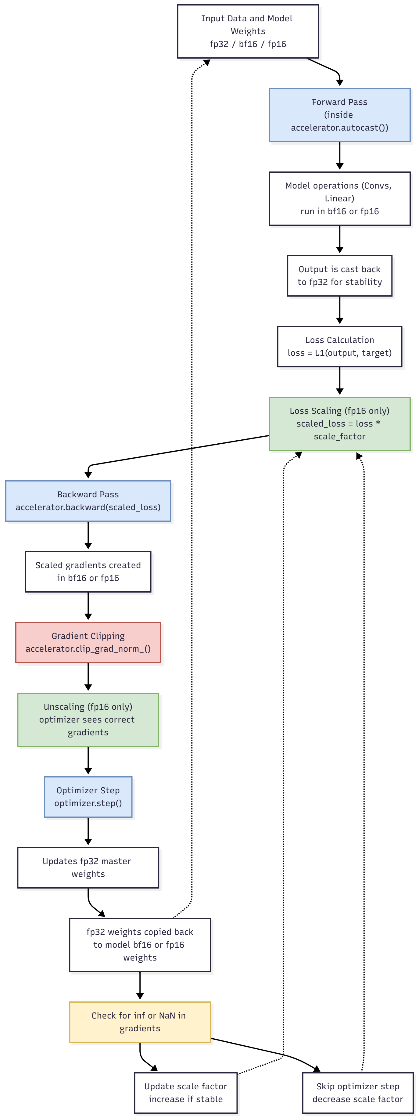
Mixed Precision Pipeline. Weights are converted between fp32 -> fp16 in P100

Progressive Training: We don’t use the full noise schedule from the start. Instead, we begin with a small number of discrete timesteps (num_scales) and gradually increase it. This curriculum learning approach is more stable to learn coarse features first before refining the details. The number of scales is increased quadratically with the training step.

Note: P100 doesn’t support bf16.

1
def main():
2
    config = Config()
3
    loss_history, lr_history, scales_history = [], [], []
4
    dataset = get_dataset(config)
5
    train_dataloader = DataLoader(dataset, batch_size=config.batch_size, shuffle=True, num_workers=2)
6
    accelerator = Accelerator(mixed_precision="fp16")
7
    os.makedirs(config.output_dir, exist_ok=True)
8

9

10
    student_model = UNetModel(image_size=config.image_size, in_channels=config.in_channels, model_channels=config.model_channels, out_channels=config.out_channels, num_res_blocks=config.num_res_blocks, attention_resolutions=config.attention_resolutions, dropout=config.dropout, channel_mult=config.channel_mult, num_heads=config.num_heads, use_fp16=accelerator.mixed_precision=="fp16")
11
    target_model = UNetModel(image_size=config.image_size, in_channels=config.in_channels, model_channels=config.model_channels, out_channels=config.out_channels, num_res_blocks=config.num_res_blocks, attention_resolutions=config.attention_resolutions, dropout=config.dropout, channel_mult=config.channel_mult, num_heads=config.num_heads, use_fp16=accelerator.mixed_precision=="fp16")
12

13
    target_model.load_state_dict(student_model.state_dict())
14
    for param in target_model.parameters(): param.requires_grad = False
15

16
    optimizer = torch.optim.AdamW(student_model.parameters(), lr=config.learning_rate)
17
    lr_scheduler = get_scheduler(config.lr_scheduler_type, optimizer=optimizer, num_warmup_steps=config.lr_warmup_steps, num_training_steps=config.num_train_steps)
18

19
    student_model, target_model, optimizer, train_dataloader, lr_scheduler = accelerator.prepare(student_model, target_model, optimizer, train_dataloader, lr_scheduler)
20

21
    karras_denoiser = KarrasDenoiser()
22
    l1_loss = nn.L1Loss(reduction="none")
23
    global_step, resume_step = 0, 0
24

25

26
    if config.resume_from_checkpoint:
27
        path = None
28
        if config.resume_from_checkpoint != "latest": path = config.resume_from_checkpoint
29
        else:
30
            dirs = [d for d in os.listdir(config.output_dir) if d.startswith("checkpoint")] if os.path.exists(config.output_dir) else []
31
            if dirs: dirs.sort(key=lambda x: int(re.search(r"-(\d+)", x).group(1))); path = os.path.join(config.output_dir, dirs[-1])
32
        if path and os.path.exists(path):
33
            accelerator.print(f"Resuming from checkpoint {path}"); accelerator.load_state(path)
34
            resume_step = 30000
35
            global_step = resume_step
36
            accelerator.print(f"Manually set resume step to: {global_step}")
37
        else: accelerator.print("No checkpoint found. Training from scratch.")
38

39
    progress_bar = tqdm(total=config.num_train_steps, initial=resume_step, disable=not accelerator.is_local_main_process, desc="Training")
40

41

42
    while global_step < config.num_train_steps:
43
        for step, batch in enumerate(train_dataloader):
44
            if global_step >= config.num_train_steps: break
45

46
            num_scales = int(np.ceil(np.sqrt((global_step / config.num_train_steps) * (config.end_scales**2 - config.start_scales**2) + config.start_scales**2)))
47
            num_scales = min(num_scales, config.end_scales)
48

49
            student_model.train()
50
            optimizer.zero_grad()
51

52
            clean_images = batch["images"]
53
            noise = torch.randn_like(clean_images)
54

55
            loss = karras_denoiser.consistency_losses(model=student_model, x_start=clean_images, num_scales=num_scales, target_model=target_model, loss_fn=l1_loss, noise=noise)
56

57
            accelerator.backward(loss)
58
            optimizer.step()
59
            lr_scheduler.step()
60

61
            with torch.no_grad():
62
                for student_p, target_p in zip(student_model.parameters(), target_model.parameters()):
63
                    target_p.copy_(config.ema_decay * target_p + (1 - config.ema_decay) * student_p)
64

65
            progress_bar.update(1)
66
            global_step += 1
67

68
            logs = {"loss": loss.detach().item(), "lr": lr_scheduler.get_last_lr()[0], "scales": num_scales, "step": global_step}
69
            progress_bar.set_postfix(**logs)
70

71
            loss_history.append(logs["loss"])
72
            lr_history.append(logs["lr"])
73
            scales_history.append(logs["scales"])
74

75
            if accelerator.is_main_process and global_step % config.save_checkpoint_steps == 0:
76
                old_checkpoints = [d for d in os.listdir(config.output_dir) if d.startswith("checkpoint")]
77
                save_path = os.path.join(config.output_dir, f"checkpoint-{global_step}")
78
                accelerator.save_state(save_path)
79
                for old_ckpt in old_checkpoints: shutil.rmtree(os.path.join(config.output_dir, old_ckpt))
80

81

82
    if accelerator.is_main_process:
83
        student_model_final = accelerator.unwrap_model(student_model)
84
        torch.save(student_model_final.state_dict(), f"{config.output_dir}/consistency_model_final.pth")
85
        print("Final model saved.")
86

87
        @torch.no_grad()
88
        def sample(model, num_samples=64):
89
            model.eval()
90
            sigmas = torch.tensor([karras_denoiser.sigma_max]).to(accelerator.device)
91
            x_t = torch.randn(num_samples, config.in_channels, config.image_size, config.image_size, device=accelerator.device) * sigmas
92
            denoised_images = karras_denoiser.denoise(model, x_t, sigmas)
93
            denoised_images = (denoised_images.clamp(-1, 1) + 1) / 2
94
            save_image(denoised_images, f"{config.output_dir}/sample.png", nrow=int(math.sqrt(num_samples)))
95
            print(f"Saved {num_samples} samples to {config.output_dir}/sample.png")
96

97
        sample(student_model_final)
98

99
        return loss_history, lr_history, scales_history
100

101
    return None, None, None

We checkpoint the model every 1000 steps to ensure that we can have a backup whenever the training fails.

Part 5 - Inference

5.1 - Single Step Inference

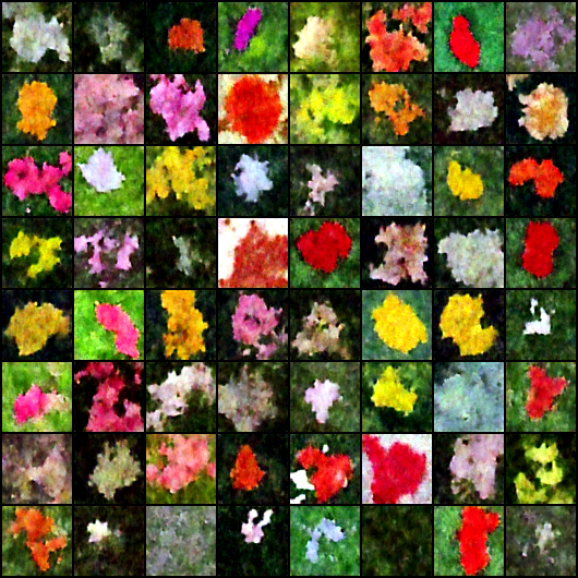
This is the fastest method. We start with pure random noise $x_T$ (scaled by $\sigma_{max}$) and pass it through the model just once.

1
karras_denoiser = KarrasDenoiser()
2
sigmas = torch.tensor([karras_denoiser.sigma_max]).to(device)
3
x_t = torch.randn(num_samples, 3, 64, 64, device=device) * sigmas
4

5
# single step
6
denoised_images = karras_denoiser.denoise(model, x_t, sigmas)

Output:

5.2 - Multi Step Inference

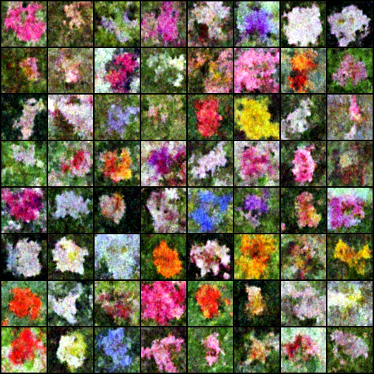
For better quality, we use the refinement process from the paper. In this, we alternate between denoising and adding a small amount of noise back in, allowing the model to correct its own mistakes.

Initial Denoise: Get an initial image $x$ from pure noise $x_T$.
Refinement Loop (N-1 times):
- Add a controlled amount of noise back to $x$. The amount of noise is $\sqrt{\tau_n^2 - \epsilon^2}$.
- Denoise the newly noised image from its corresponding noise level $\tau_n$.

1
T = karras_denoiser.sigma_max
2
    epsilon = karras_denoiser.sigma_min
3

4
    # create schedule of timesteps for the refinement loop
5
    tau_schedule = torch.exp(torch.linspace(math.log(T), math.log(epsilon), num_steps)).to(device)
6
    tau_schedule = tau_schedule[1:]
7

8
    with torch.no_grad():
9
        x_T = torch.randn(num_samples, 3, 64, 64, device=device) * T
10

11
        x = karras_denoiser.denoise(model, x_T, torch.tensor(T, device=device))
12

13
        # refinement loop
14
        for tau_n in tau_schedule:
15
            z = torch.randn_like(x)
16
            noise_scale = (tau_n**2 - epsilon**2).clamp(min=0).sqrt()
17
            x_tau_n = x + noise_scale * z
18
            x = karras_denoiser.denoise(model, x_tau_n, tau_n)

Output (25 steps):

#ai

#diffusion models

#image generation

#consistency

#models